Most private market forecasting stops at the capital call: when the funds will draw, and how much. That ground is well covered, and the models for it are mature.
It is still only half a liquidity plan. What a principal actually asks is whether the cash will be there, in the right entity and the right currency, on the day the notice lands. Answering that means netting projected calls against what is coming in, and knowing where cash sits inside the structure.
This guide covers the five assumptions behind any call forecast, why calibrating by vintage matters, how to stress the result, and how to build the other half of the plan.
What is capital call forecasting?
Capital call forecasting projects when each private fund will draw on your commitment and how much it will draw each time. It converts an unfunded commitment, which carries no fixed payment date, into an expected schedule of cash going out.
On its own that is half a forecast. The other half projects what comes back: fund distributions, bond coupons, rent, maturities. Net the two and you get the number a principal actually asks for, which is how much cash to hold and where.
Two forecasts, one plan
- Cash out: capital calls across every closed-end commitment, by quarter and by month.
- Cash in: distributions, coupon payments, bond maturities, rent, loan repayments.
- The plan: the two netted, in the entity and currency where the cash is actually needed.
Why capital calls resist a calendar
Committing to a fund is not the same as paying for it. You sign for €10m, and the manager draws it over several years as deals appear. The manager sets that pace, not you. Nothing about it is fixed in advance, which is exactly what makes it hard to plan around.
Four things make the timing slippery.
The manager controls the schedule. Calls follow deal flow. A quiet year of sourcing means a quiet year of calls, then two deals close in one quarter and a year's worth of capital is drawn at once.
The notice period is short. ILPA's model partnership agreement sets drawdown notice at no less than 10 business days before payment is due (ILPA Model LPA). Individual funds set their own terms, and the first call after a closing is often shorter. Ten business days is enough to move cash you already hold. It is not enough to sell an illiquid asset at a sensible price.
Valuations arrive late. Private funds report net asset value quarterly, and ILPA's model agreement allows 45 days after quarter end to deliver the unaudited report. The number in front of you describes a position that has already moved.
The J-curve runs the wrong way early. In a fund's first years, capital goes out for deals and fees while nothing has been sold. Calls and distributions do not offset each other until well into the fund's life.
The scale is not small. Global private equity dry powder, which Preqin defines as capital committed to a fund minus the amount the manager has called, stood at $2.184 trillion as of 31 March 2025 (S&P Global Market Intelligence, analysing Preqin data). Among US family offices, alternatives now make up 54% of the portfolio, split 27% private equity, 18% real estate and 3% private debt (UBS Global Family Office Report 2025). Most of a family's wealth now sits in assets that pay on someone else's schedule.
The five assumptions that drive the forecast
Every model of private fund cash flows rests on a short list of inputs. Get these right and the schedule is useful. Guess at them and it is decoration.
| Assumption | What it sets | Why it moves the answer |
|---|---|---|
| Fund life | How many years the fund runs before wind-up | Stretches or compresses the whole schedule |
| Call schedule shape | Whether calls are front-loaded or spread evenly | Decides how much cash you need in years one to three |
| Investment horizon | The period over which calls are made | Sets how quickly the commitment is drawn down |
| Distribution start year | When cash begins coming back | Determines how long you fund calls unaided |
| Target return | The IRR or TVPI the fund is modelled to reach | Scales the size of distributions |
The standard reference here is the Takahashi-Alexander model, often shortened to the TA model. Dean Takahashi and Seth Alexander wrote it at the Yale University Investments Office in January 2001, and it was published in the Journal of Portfolio Management the following year. It projects calls, growth and distributions across a fund's life from this kind of small parameter set, and it has held up for over twenty years.
You will also see it called the Yale Model. That name is best avoided here. It usually refers to the endowment allocation approach associated with David Swensen, which is about how much to hold in alternatives, not when the cash moves. Two different ideas that happen to share an institution, and Takahashi worked on both.
It has two practical limits worth naming. It steps in full years, and real portfolios move within them. And it expects you to set assumptions by hand, which is fine for one fund and unmanageable across thirty.
Calibrate by vintage, not by average
Here is where most forecasts quietly go wrong. One assumption gets applied to every fund in the book.
A 2020 fund and a 2025 fund are at opposite ends of their lives. The 2020 fund has probably called most of its capital and may be distributing. The 2025 fund has years of calls ahead. Applying an average call rate to both understates the near-term demand from the young fund and overstates it from the old one. The two errors do not cancel out, because they land in different quarters.
Calibrating by vintage year fixes this. The model reads when each fund started and adjusts its remaining call and distribution profile accordingly. It costs nothing in effort once the vintage is recorded and removes an entire class of error.
A quick test of your own forecast
Pull your two oldest and two newest fund commitments. Do they carry the same call rate assumption? If they do, your near-term cash requirement is wrong, and probably understated.
Work backwards from a target
Setting assumptions forwards is guesswork dressed as precision. Nobody knows a fund's exact call schedule.
The more honest approach runs the other way. State the return you are underwriting the fund to reach, a goal TVPI or a goal IRR, and let the model solve for the cash flow path that gets there. You are no longer inventing a number you cannot know. You are testing what has to be true for the investment case to hold.
The two goals pull against each other. A high IRR wants capital back early. A high TVPI wants capital compounding longer. Deciding which you weight, or holding a balance between them, is a real allocation decision, and making the model state it out loud is useful in itself.
Stress it before the market does
A base case is not a plan. The quarter that hurts is the one where calls come early and distributions do not arrive.
Shock the two variables independently:
- Calls arrive faster than expected. Raise the call rate by 50% or 75% and see which quarter breaks.
- Distributions disappoint. Cut expected distributions by half and check how long you can fund calls without them.
- Both at once. This is the downside case that actually matters.
Run upside, base and downside side by side. Read the worst quarter, not the average, because the average never turns up. Save each set of assumptions as a named scenario so next quarter is a rerun rather than a rebuild, and so anyone can see what changed and why.
Treat projected distributions as the weakest line in the whole model. Calls follow deployment, which the manager broadly controls. Distributions depend on selling into whatever market exists at the time. In a slow exit market, distributions slip and calls do not.
When distributions stall, secondaries are the release valve
If distributions do not arrive and calls keep coming, selling a fund interest on the secondary market is the way out. That has stopped being a distress signal and become an ordinary portfolio tool.
The volumes show it. The global secondary market reached $240 billion in 2025, up 48% on the year and the largest on record, split $125 billion LP-led and $115 billion GP-led (Jefferies). Jefferies expects annual volume to approach $300 billion within the next one to two years.
Two things follow for a family office. You have a real exit if the liquidity plan goes wrong, which is worth knowing before you need it. And the market puts an independent price on fund interests that would otherwise be valued only by the manager holding them.
Neither makes secondaries a base case. Selling into the secondary market usually means accepting a discount to carrying value, so it belongs in the plan as the fallback, not as a projected inflow.
The half of the plan everyone skips
Most writing on this subject stops at projected calls. That leaves the plan half-built, because a call is only a problem if nothing is coming in to meet it.
Some of your inflows are far more predictable than any private fund model.
Fixed income is knowable to the day. For every bond you hold, the coupon rate, payment frequency and maturity date are already contracted. That is not a projection, it is arithmetic. You can say what income arrives in March 2028 and which holdings pay it. A five-year maturity schedule shows which bonds roll off and when, which is both a source of cash and a reinvestment decision.
Rent is contracted. Each lease has a term, a rent and an expense profile. What matters is comparing expected against actual, because a tenant paying quarterly when the lease says monthly, or paying late, changes your cash position even though the lease has not changed.
Loan repayments amortise on a schedule. Structured borrowings can be modelled exactly, including rate changes and early repayments.
Set these against your projected calls and the picture changes. A quarter that looked tight on calls alone may be comfortable once a bond matures in the same month. Forecasting calls without forecasting these inflows produces a number that is technically correct and practically useless.
Cash in the group is not cash you can use
One more gap closes the plan. A group-level cash total tells you very little if the cash sits in the wrong place.
Families hold assets through layered structures: holding companies, trusts, partnerships, several people owning slices of each. The commitment sits with one entity. The cash may sit with another. Moving between them may take time, trigger tax, or need approvals.
So the useful view apportions ownership through the structure, showing each owner's real share of what sits underneath, and then splits it by liquidity. That answers the question a group total cannot: not does the family have €5m, but does the entity that owes the call have €5m it can use this month, in this currency.
Why the spreadsheet gives out
Most family offices start in Excel, and for a handful of commitments it works. It stops working in predictable ways.
- It does not recalculate. A call lands, a NAV updates, and the forecast still shows last quarter's world. The model is a photograph, not a live view.
- One person owns it. The analyst who built it is the only one who fully understands it, which is a genuine risk when they leave.
- The assumptions are buried. When this quarter's forecast differs from last quarter's, nobody can say whether the portfolio changed or someone changed a cell.
- It does not scale. Thirty funds across several entities and currencies is where hand-maintained models fall apart.
The fix is not a better spreadsheet. It is putting the forecast next to the data that feeds it, so it updates when the portfolio does.
How Asora forecasts capital calls
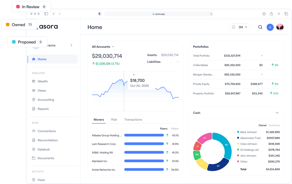
Asora builds the forecast on the same records that already track your commitments, so the projection moves when the portfolio moves. No re-keying, no separate model to maintain.
Three levels of control. Simple, advanced and expert modes. Expert lets you pick the projection model, choose whether assumptions apply flat across the book or calibrate to each fund's vintage, and set a goal TVPI or goal IRR with the balance you want between them. You set the call schedule shape, the investment horizon and the year distributions begin.
Scenarios you keep. Save any set of assumptions as a template and reuse it. Run sensitivity tests that shock call rates and distribution rates to build upside, base and downside cases.
Output at the granularity of the decision. A ten-year projection of calls, distributions and the resulting TVPI and IRR path. Drill into a single fund to see the years it is expected to call and the year distributions begin. For the coming year, break the schedule down by quarter and by month, which is the horizon you actually hold cash against.
The record underneath. The private equity dashboard tracks value, capital calls, income and remaining commitments beside DPI, TVPI, RVPI and IRR, with J-curve analysis and breakdowns by vintage, geography and sector. Where a manager sends one combined transaction, you can split it, so part is recorded as a capital call and part as a recallable distribution rather than being forced into one bucket.
Both sides of the ledger. Fixed income income projections use each holding's coupon, payment frequency and maturity date to show expected income by month, with a five-year maturity schedule. Property leases track expected against actual income and expenses. The loan calculator builds full amortisation schedules and recalculates when terms change.
Where the cash sits. Look-through net worth apportions ownership across every entity in the structure and splits the result by liquidity, owner, currency and asset class, so you can see which entity holds usable cash.
Sources
- ILPA, Model Limited Partnership Agreement (Whole of Fund) Term Sheet: drawdown notice of no less than 10 business days, and quarterly reporting within 45 days of quarter end.
- Preqin, Private capital investment terms: dry powder defined as capital committed to a fund minus the amount called by the general partner.
- S&P Global Market Intelligence, Private equity dry powder recedes from all-time highs (11 December 2025): global private equity dry powder of $2.184 trillion as of 31 March 2025, from an analysis of Preqin data.
- UBS, Global Family Office Report 2025: US family office allocations to alternatives, private equity, real estate and private debt.
- Jefferies, 2025 Global Secondary Market Review: record secondary volume of $240 billion in 2025, split between LP-led and GP-led transactions.
- Takahashi, D. and Alexander, S., Illiquid Alternative Asset Fund Modeling, Yale University Investments Office (January 2001), published in the Journal of Portfolio Management, 28(2), 2002, pp. 90–100: the standard framework for projecting private fund calls, growth and distributions.
FAQ
What is capital call forecasting?
Capital call forecasting projects when a private fund will draw on your commitment and how much it will draw each time. It turns an unfunded commitment, which has no fixed payment date, into an expected schedule of cash out. Family offices use it alongside a distribution forecast to work out how much cash they need to hold, and when.
How far in advance do you get notice of a capital call?
Notice periods are set in the fund's partnership agreement. ILPA's model agreement sets a floor of no less than 10 business days before payment is due, and many funds follow that shape, though terms vary and the first call after a closing is often shorter. Ten business days is enough to move cash you already hold, but not enough to sell an illiquid asset at a sensible price.
What assumptions drive a capital call forecast?
Five do most of the work: the fund's life, the shape of the call schedule (front-loaded or spread evenly), the investment horizon over which calls are made, the year distributions begin, and the target return. Change any one and the schedule moves. A forecast is only as good as how honestly these are set and how consistently they are applied.
What is the Takahashi-Alexander model?
The Takahashi-Alexander model, or TA model, is a framework written by Dean Takahashi and Seth Alexander in 2001 that projects a private fund's calls, growth and distributions across its life from a handful of assumptions. It remains the standard reference for private market cash flow forecasting, and is sometimes loosely called the Yale Model. Its limits are that it steps in full years and expects you to set assumptions by hand, so most practical forecasts extend it to handle intra-year timing.
Should capital calls be forecast per fund or across the portfolio?
Both, and the two answer different questions. The per-fund view tells you which manager is likely to call and when, which is what you need for the conversation with that manager. The portfolio view nets every fund together into one schedule, which is what you need for the liquidity decision. Only the portfolio view shows the quarter where three funds happen to call at once.
How do you stress test a capital call forecast?
Shock the two variables that hurt. Raise the call rate, so capital is drawn faster than expected, and cut the distribution rate, so less comes back to fund it. Run that as a downside case beside your base case and an upside case. The number that matters is not the average outcome but the worst quarter: how much cash you would need if calls came early and distributions stalled.
Why do spreadsheets fail at capital call forecasting?
They do not update. A spreadsheet forecast is a photograph of one afternoon's assumptions, and nothing in it recalculates when a call lands or a valuation changes. One person usually owns the model, which is a real risk when they leave, and the assumptions sit buried in cells, so no one can explain why this quarter's forecast differs from last quarter's.
Is forecasting distributions harder than forecasting calls?
Yes, and you should plan as if it is. Calls follow deployment, which a manager broadly controls. Distributions depend on selling assets into whatever market exists at the time, so exit timing slips in slow markets. The safe approach is to treat projected distributions as the least reliable line in your forecast and never rely on one arriving to meet a call.

.png)
 ISO 27001 Certified
 GDPR Compliant